TL;DR
Auditory attention decoding (AAD) asks which of several talkers a listener attends to, from a few seconds of brain recording such as electroencephalography (EEG). Recent side classifiers report 95–97% accuracy from 1 s of EEG; run in this paper's pipeline they fall to 40–62% on DTU, ESAA and a 255-channel dataset once the test speech is never heard in training, because they can read trial identity, eye gaze or acoustic cues instead of the brain's response to speech. CoupleFlow decides only through the time-locked coupling between a neural embedding and each candidate talker's acoustic embedding, so it is provably at chance when the recording carries no information about the speech. On content-disjoint folds of nine EEG and magnetoencephalography (MEG) datasets it outperforms linear and deep baselines trained on the same splits on seven of eight datasets at 5 s and ties the linear decoder on the eighth, its null tests stay at chance, and an evidence-accumulation law predicts accuracy at any window length from one parameter per dataset.
Abstract
When several people talk at once, the auditory cortex follows the talker a listener attends to. Auditory attention decoding (AAD) asks whether that talker can be identified from a few seconds of non-invasive brain recording, by matching the recording against the speech of each candidate talker; neuro-steered hearing devices are a potential long-term application. Recent decoders report near-perfect accuracy from a second of electroencephalography (EEG). We show that these results do not survive evaluation on unheard speech, because the decoders exploit leaked trial information, eye gaze and acoustic cues rather than the neural response to speech. We introduce CoupleFlow, a decoder that can reach its decision only through the time-locked coupling between a neural embedding and each candidate talker's acoustic embedding. It is therefore provably at chance whenever the brain signal carries no information, so no acoustic or identity shortcut can inflate its accuracy. A conditional flow-matching head adds a likelihood-ratio decision rule, the pointwise mutual information between speech and brain, which is Bayes-optimal when the recording depends only on the attended talker and cancels the bias toward acoustically typical speech. We pair the model with a leakage-free protocol: content-disjoint splits recovered from the audio itself and null tests that separate true time-locking from trial recognition. Across nine EEG and magnetoencephalography (MEG) datasets under one preprocessing pipeline, covering four languages, high-density caps, hearing-impaired listeners and a multi-talker room, CoupleFlow outperforms linear and deep baselines trained on identical splits on seven of eight datasets and ties the linear decoder on the eighth, while its nulls stay at chance. Finally, we derive an evidence-accumulation law that predicts accuracy at any window length from a single parameter per dataset, and predicts that parameter from how strongly the brain tracks speech. The law shows that fast, reliable decoding is limited by the signal-to-noise ratio of the recording, and gives the window any target accuracy requires.
The problem: high accuracies that do not survive unheard speech
Given a few seconds of a multichannel recording and the speech of \(K\) candidate talkers, a decoder must name the talker the listener attends to. The neural response to speech is weak: a linear decoder's reconstruction correlates with the attended envelope at only \(r=0.07\)–\(0.17\) on the two-talker EEG datasets studied here. It differs across listeners and is mixed with activity unrelated to the audio, while the candidates often differ in ways a decoder can exploit without reading the brain: loudness, voice, or the identity of the recording session.
AAD decoders follow two strategies. Stimulus reconstruction estimates the attended speech envelope from the EEG and selects the candidate that correlates best with it. Linear backward models and canonical correlation analysis are robust, but need tens of seconds for high accuracy, and deep nonlinear reconstructions have not changed this picture. Direct classification maps the EEG to a label, usually the side of the attended talker. Recent direct classifiers (DARNet, DBPNet, ListenNet) report 95–97% at 1 s on KU Leuven. The paper reran the authors' models in its own training pipeline:
The paper identifies the routes by which such accuracies arise without decoding attention:
- Trial identity. When training and test windows come from the same trial, EEG carries slow, trial-specific structure (electrode impedances, drifts, posture and gaze, and an attended side that is constant within the trial). A decoder that recognises which trial a window comes from knows its label without decoding attention. Splitting windows within a trial inflated the earlier decoders by 16.7–31.5 points.
- Eye gaze and lateralised artefacts. A side classifier uses no audio, so any EEG signal that differs between left and right trials helps, including eye movements toward the attended loudspeaker. On a dataset where gaze and attention were dissociated, accuracy followed gaze (Rotaru et al., 2024).
- Acoustic cues. Loudness or spectral differences can mark the attended talker without any neural input. In the MAESTRO room recordings the attended talker is always the loudest, by 3–18 dB.
- Repeated stimuli. Most datasets play the same stories to every listener, and some replay them, so holding out trials does not hold out speech.
- Wrong timing. In one widely used dataset (NJU) the EEG is not time-aligned with the audio at any offset, so results on it cannot reflect speech tracking.
The two kinds of leakage differ greatly in size. Retraining every model on KU Leuven and DTU with a split that shares stories across folds changes 5-s accuracy by only −0.3 to +2.0 points, because each of these decoders reaches its decision through the neural response to the candidate audio. Splitting windows within a trial is the large effect. What inflates AAD accuracy is evaluating on windows of trials seen in training; content-disjoint folds rule out both.
Method: CoupleFlow
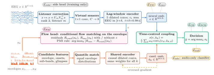
Inputs and the two paths
A decision window of \(T\) seconds (\(L=64T\) samples at 64 Hz) gives the recording \(x\in\mathbb{R}^{C\times L}\) of \(C\) channels, the speech envelopes \(a_1,\dots,a_K\in\mathbb R^{L}\) of \(K\) candidate talkers, and the index \(y\) of the attended one. A neural path embeds the recording and an acoustic path embeds each candidate, both as time series of the same size. The two paths meet only in the coupling score, which makes the decision.
Neural path. A listener correction \(x\mapsto x+U_m V_m^{\top}x\) (rank 2, 256 parameters per listener \(m\), with \(U_m\) initialised at zero) absorbs individual differences such as head shape and cap placement without fitting a separate model to each listener's few minutes of data. Virtual sensors (a \(1{\times}1\) convolution, \(C\to8\)) reduce the channels to a few learned spatial filters, as backward models do, and a lag-window encoder (five dilated convolutions) produces the neural embedding \(e\in\mathbb{R}^{16\times L}\). Each time step of \(e\) sees only the EEG that follows the corresponding sound, from a lag \(\delta\in\{0,125\}\) ms on, which is where a cortical response to that sound must lie.
Acoustic path. Each candidate is described by its envelope and onsets and, where the audio is available, sub-band envelopes and glimpsed/masked channels that mark where the talker is louder or quieter than the competing one. In training, a quantile match gives the candidates' envelopes identical value distributions, which removes loudness and level cues. A shared encoder with the same weights for every candidate maps each one to an embedding \(\hat a_k\in\mathbb{R}^{16\times L}\). It sees only past audio, so the brain response it is compared with must follow the sound.
The coupling score
The coupling score measures how each candidate's embedding co-varies in time with the neural embedding:
where \(e_{\cdot d}\in\mathbb R^{L}\) is dimension \(d\) of \(e\) over time and \(\bar e_d\) its time average (likewise for \(\hat a\)). Each fraction is the Pearson correlation over time between one neural and one acoustic dimension; the weights \(\omega_d\) and the temperature \(\tau\) are learned. Candidate \(k\) scores
Because the correlation removes each dimension's time average, a neural embedding that does not vary in time gives every candidate the score 0. The audio alone then cannot favour any candidate, and the decoder is at chance whenever the EEG carries no information about the speech:
Proposition 1 (null calibration). A decoder gives candidate \(k\) a score \(s_k\) and predicts \(\hat y=\arg\max_k s_k\); a tie for the maximum counts as an error. Assume (a) \(s_k=g(x,a_k)\) for one function \(g\) shared by all candidates; (b) \(H_0\): \(x\) is independent of \((y,a_{1:K})\); (c) given \(y\), the joint law of \(a_{1:K}\) is invariant to permuting the candidate indices. Then under \(H_0\), \(P(\hat y=y)\le 1/K\).
Eq. 1 satisfies (a), and the across-trial and circular nulls described below realise (b). For the time-centred score, a time-constant embedding yields \(s_k=0\) for all \(k\), a tie, hence an error: the acoustic pathway alone cannot exceed chance. Assumption (c) holds exactly for the same-talker candidate set (the negative is the attended talker's own speech) and approximately for the competing set in counterbalanced designs.
Flow head and the PMI decision rule
Alongside the coupling score, the flow head, a conditional flow-matching network, learns to generate the attended envelope from \(e\). Flow matching joins Gaussian noise \(\varepsilon\sim\mathcal N(0,I_L)\) to the data along the straight path \(a^{(u)}=(1-u)\,\varepsilon+u\,a\), indexed by the flow time \(u\in[0,1]\), whose velocity is \(a-\varepsilon\), and trains a network \(v_\theta(a^{(u)},u,c)\) with parameters \(\theta\) and condition \(c\) to predict that velocity:
The condition is \(c=e\); with probability 0.2 it is set to zero and flagged as absent (\(c=\varnothing\)), as in classifier-free guidance, so one network defines both \(p(a\mid x)\) (with \(c=e\)) and \(p(a)\) (with \(c=\varnothing\)). At test time each candidate is scored by its residuals \(R_{\rm cond}(a_k)=\mathbb E_{u,\varepsilon}\|v_\theta(a_k^{(u)},u,e)-(a_k-\varepsilon)\|^2\) and \(R_{\rm unc}(a_k)\), the same with \(c=\varnothing\). The expected flow-matching residual acts as a surrogate for the negative log-likelihood, so how much the recording lowers the error on \(a_k\) is a proxy for the pointwise mutual information, and picking the candidate with the largest PMI is a second decision rule:
Proposition 2 (PMI is Bayes-optimal). Let \(p(a)\) be the density of the attended envelope \(a_y\) and \(p(a\mid x)\) its density given the recording, and \(\mathrm{PMI}(a;x)=\log p(a\mid x)-\log p(a)\). Assume (a) the recording depends on the candidates only through the attended one, \(p(x\mid a_{1:K},y)=p(x\mid a_y)\); (b) \(y\) is uniform on \(\{1,\dots,K\}\) and independent of \(a_{1:K}\). Then the maximum a posteriori (MAP) decision is \(\hat y=\arg\max_k\mathrm{PMI}(a_k;x)\). Scoring by \(\log p(a_k\mid x)\) instead adds \(\log p(a_k)\), a term that depends on the audio alone.
Since \(\log p(a_k)\) cancels, no candidate can win by being typical speech, and a network that ignores \(e\) scores every candidate 0, as Eq. 1 does. Unattended speech is weakly tracked, so assumption (a) is an approximation; the matched and same-talker candidate sets partly address it.
Training objective
The model is trained end to end on
The decoding terms ask for the right decision, through cross-entropy over the candidates and a contrastive (InfoNCE) term that matches each window's EEG to its own attended speech among all windows of the batch. The anti-shortcut terms close routes around the brain: a hinge requires the attended speech to score higher with its own recording than with another window's, an audio-only adversary, through a reversed gradient, strips acoustic cues to the attended talker from the shared encoder, and a VICReg term keeps the neural embedding from collapsing. The density term trains the flow head. The auxiliary terms train a side head, which predicts the attended side from the EEG in training only, and an envelope read-out that reports tracking; neither enters a reported decision. The weights (\(\lambda_{\rm NCE}=1\), \(\lambda_{\rm null}=0.5\), \(\lambda_{\rm adv}=\lambda_{\rm FM}=\lambda_{\rm side}=0.3\), \(\lambda_{\rm VIC}=0.1\), \(\lambda_{\rm env}=0.2\)) were set once and are identical for every dataset. The part that makes the decision has 25,689 shared parameters plus 256 per listener; the full model has 126,607–148,879 parameters per dataset.
Protocol: content-disjoint folds and null tests
Test speech is never heard in training, and every accuracy comes with nulls that make the EEG uninformative.
Content-disjoint folds recovered from the audio
Most datasets play the same stories to every listener, and KU Leuven replays each story pair five times per listener, so a trial split puts the same speech in training and test. The releases lack a reliable stimulus key, so the paper finds the trials that contain the same speech by correlating their envelopes:
- Every candidate envelope is averaged to 8 Hz and cut into non-overlapping 10-s chunks; each chunk is correlated with every 10-s window, at every 1/8-s offset, of every other envelope. Pairs with \(r>0.9\) are candidates.
- Each candidate pair is re-correlated at 64 Hz over the full overlap at the implied offset (±1/8 s) and kept if \(r>0.95\). Two envelopes are linked if both stages pass.
- Trials are the nodes of a graph, with an edge whenever any of their envelopes are linked. Its connected components, found with union–find, are the content groups, and each test fold is a union of whole groups (\(\min(5,\text{groups})\) folds).
Proposition 4 (content disjointness). No test stream is linked to any training or validation stream.
A copy of one recording gives \(r\approx1\) (every kept link has \(r\ge0.964\)), while the 64-Hz correlation at the best match of a 10-s chunk in another group has a median of at most 0.53 per dataset. The grouping matters: the 320 KU Leuven trials form 4 groups, and Fuglsang’20 numbers its files per listener, yet its 1401 trials contain only 4 distinct contents.
Candidate sets
- Competing (comp.): the attended vs. the other talker.
- Matched: the same pair after quantile matching, which removes loudness cues.
- Same-talker (match–mismatch, mm): the attended speech vs. the same talker's speech from another window of the trial; the only task for single-talker data.
Null tests
- Across-trial permutation. The recording is replaced by another trial's recording of the same listener (20 permutations at 5 s and 3 at other windows; when a listener has a single test trial, windows of that trial are permuted instead).
- Circular shift. At 5 s, the trial's own recording shifted by at least 2 s (5 random shifts). This keeps trial identity but breaks time-locking, so a decoder that recognises the trial rather than the response would stay above chance.
- Lag control. The encoder reads EEG from before the sound, which cannot be a response to it.
Checkpoints are selected on validation contribution, accuracy minus the across-trial null, which rewards what the brain adds rather than what the audio or trial identity allows. The lag \(\delta\) is the one hyperparameter set per dataset, on validation accuracy only.
Baselines
One decoder from each main family, all trained on the same folds, windows and inputs and stopped early on validation data: the per-listener linear backward model (ridge regression from EEG at lags 0–250 ms), still the standard for AAD; VLAAI, a deep reconstruction model trained across listeners; and a dilated-convolution match–mismatch model (Dil. MM), which, like CoupleFlow, compares the EEG with each candidate directly. A recursive decoder (DECAF) stays near chance on the two-talker sets and is reported only in the paper's appendix.
Results
Main comparison
At 5 s CoupleFlow is best on seven of eight datasets. Its margin over the strongest baseline is +6.8 points on KU Leuven, +3.8 on DTU, +2.3 on Fuglsang’20, +3.8 on ESAA, +3.9 on the 255-channel set, +8.9 on SparrKULee and +2.8 on MEG-MASC. On Broderick it ties the per-listener linear decoder (−0.1, within one seed s.d.) and stays within one point of it at every window. On the five other two-talker EEG sets the margin grows from 1 to 20 s, to at most +8.5 points; on the single-talker match–mismatch sets it is largest at 1 s (at least 10.9 points). On unseen listeners (leave-one-listener-out, LOSO: listener and content held out together) CoupleFlow keeps 2.0–8.3 points over the pooled linear model wherever either transfers.
Table 1. Accuracy (%) of CoupleFlow (Ours) and the baselines at 1, 5 and 20 s on the content-disjoint folds (every model trained and tested on the same folds), and on unseen listeners (LOSO: listener and content held out, 5 s) against the pooled linear backward model. comp.: attended vs. competing talker; mm: match–mismatch. Ours: mean of 3 seeds (s.d. 0.0–1.8 at 5 s); LOSO: one seed. Bold: best per group. CoupleFlow's EEG-shuffle nulls lie in [49.7, 50.5] up to 10 s.
| Dataset | task | 1 s | 5 s | 20 s | LOSO, 5 s | ||||||||||
|---|---|---|---|---|---|---|---|---|---|---|---|---|---|---|---|
| Linear | VLAAI | Dil. MM | Ours | Linear | VLAAI | Dil. MM | Ours | Linear | VLAAI | Dil. MM | Ours | Linear | Ours | ||
| KU Leuven | comp. | 57.0 | 56.9 | 55.3 | 60.5 | 64.9 | 63.8 | 65.9 | 72.7 | 75.1 | 73.0 | 78.2 | 86.7 | 59.7 | 68.0 |
| DTU | comp. | 59.1 | 57.5 | 56.0 | 61.4 | 72.4 | 64.8 | 69.1 | 76.2 | 86.1 | 74.1 | 83.7 | 90.6 | 64.0 | 70.4 |
| Fuglsang’20 | comp. | 63.4 | 60.6 | 57.9 | 63.8 | 77.3 | 68.9 | 73.0 | 79.6 | 91.9 | 81.7 | 89.0 | 93.3 | 67.5 | 73.7 |
| ESAA | comp. | 61.3 | 58.3 | 57.5 | 63.2 | 74.1 | 66.4 | 70.6 | 77.9 | 87.6 | 78.8 | 84.7 | 90.6 | 66.1 | 68.6 |
| KUL-255ch | comp. | 57.0 | 55.9 | 54.7 | 58.9 | 65.5 | 62.1 | 65.0 | 69.4 | 76.2 | 72.1 | 77.6 | 83.0 | 64.0 | 66.0 |
| Broderick | comp. | 56.5 | 51.0 | 50.5 | 55.8 | 63.7 | 52.2 | 52.3 | 63.6 | 75.9 | 53.1 | 54.4 | 75.2 | 49.2 | 50.1 |
| SparrKULee | mm | 61.8 | 59.9 | 62.6 | 73.5 | 76.3 | 70.5 | 83.3 | 92.2 | 90.5 | 83.9 | 96.4 | 99.3 | – | 85.9 |
| MEG-MASC | mm | 72.7 | 71.0 | 72.0 | 83.7 | 92.0 | 89.1 | 96.2 | 99.0 | 99.4 | 98.6 | 100.0 | 100.0 | – | 95.0 |
An evidence-accumulation law
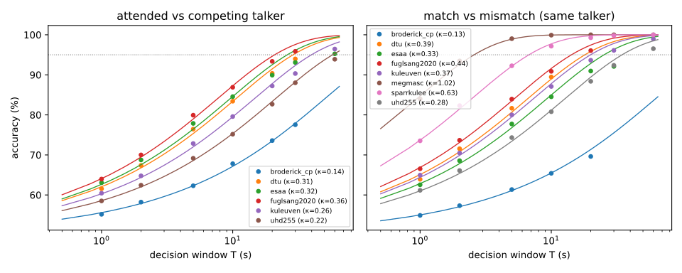
Prop. 3 of the paper models a decision that compares a decoder output's correlations with the attended and the other (competing, or match–mismatch) envelope over a window of \(T\) s that holds \(n_{\rm eff}=fT\) effectively independent samples. With \(\Delta\zeta=\zeta_{\rm att}-\zeta_{\rm neg}\) the margin between the Fisher-transformed population correlations,
and accuracy \(p\) needs \(T_p=(\Phi^{-1}(p)/\kappa)^2\) s. If the output is a signal plus independent noise with per-sample signal-to-noise ratio (SNR) \(\sigma\), then for small correlations \(\kappa^2\propto\sigma/(1+\sigma)\). \(\kappa\) is therefore a single, window-independent figure of merit: model quality and training data act through the noiseless correlation, and recording quality through \(\sigma\).
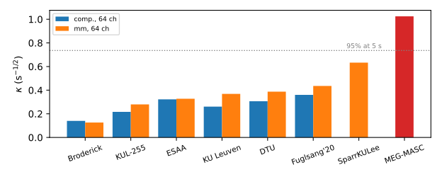
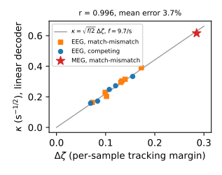
One \(\kappa\) per curve fits all 14 dataset–task curves from 1 to 60 s with mean absolute error 0.2–1.8 points, and 0.4–2.0 points when predicting a held-out window. EEG gives \(\kappa=0.13\)–\(0.63\) (\(T_{95}\), the window for 95% accuracy, = 7–170 s); MEG gives 1.02 (\(T_{95}\approx2.6\) s). With one effective rate \(f=9.7\) samples/s, \(\kappa=\sqrt{f/2}\,\Delta\zeta\) fits all 14 dataset–task values of the linear decoder (\(r=0.996\)), and MEG lies on the same line as EEG: its advantage is a per-sample signal-to-noise effect (whether the sensor or MEG-MASC's clean synthetic speech raises tracking, the paper cannot say). The law also separates task from recording: a competing talker is weakly tracked, and the predicted ratio \(\kappa_{\rm comp}/\kappa_{\rm mm}=1-\gamma\), with \(\gamma\) the ignored-talker ratio, holds on all six two-talker datasets, so the match–mismatch task raises \(\kappa\) by a factor 1.05–1.38, not more. For 95% at 5 s, EEG would need \(\kappa\approx0.74\), which only the MEG data reach. Using all native channels raises \(\kappa\) from 0.140 to 0.181 (Broderick) and from 0.190 to 0.224 (253 channels).
Envelope tracking
CoupleFlow's envelope read-out, an auxiliary head evaluated on the stricter content-disjoint folds, tracks the attended envelope better than the per-listener backward model on six of eight datasets.
Table 2. Envelope tracking \(r\) with the attended and the competing envelope. Linear: per-listener backward model, held-out trials. Ours: linear read-out of the neural embedding (\(\mathcal L_{\rm env}\)), 5-s test windows, content-disjoint folds, mean of 3 seeds.
| Dataset | Linear (trials) | Ours (5 s) | ||
|---|---|---|---|---|
| ratt | rcomp | ratt | rcomp | |
| KU Leuven | 0.099 | 0.027 | 0.133 | 0.024 |
| DTU | 0.130 | 0.023 | 0.142 | 0.025 |
| Fuglsang’20 | 0.171 | 0.018 | 0.148 | 0.006 |
| ESAA | 0.139 | 0.019 | 0.136 | 0.021 |
| KUL-255ch | 0.101 | 0.018 | 0.115 | 0.024 |
| Broderick | 0.073 | 0.003 | 0.082 | 0.048 |
| SparrKULee | 0.132 | – | 0.172 | – |
| MEG-MASC | 0.278 | – | 0.396 | – |
The PMI rule removes the audio prior
The prior-free PMI rule beats conditional likelihood by 5–25 points on every dataset, while the audio prior alone is near chance (47.0–50.9%), as Prop. 2 predicts. Conditioned on the brain, the attended talker's flow residual is lower than the competing talker's (\(\Delta R_{\rm cond}>0\) on all datasets), while the unconditional residuals are nearly equal: the attention effect lies mainly in the brain-conditioned term.
Table 3. Flow-head decision rules at 5 s (%): prior-free PMI, conditional likelihood only, audio prior only, and the PMI rule's EEG-shuffle null. \(\Delta R=R(\text{comp.})-R(\text{att.})\) for the conditional (\(R_{\rm cond}\)) and unconditional (\(R_{\rm unc}\)) residuals; for SparrKULee and MEG-MASC the negative is the mismatched window. Seed 0. NH/HI: normal-hearing/hearing-impaired listeners; zh: Mandarin.
| Dataset | PMI | log p(a|x) | log p(a) | null | ΔRcond | ΔRunc |
|---|---|---|---|---|---|---|
| KU Leuven | 69.8 | 51.8 | 47.0 | 50.3 | +0.003 | −0.012 |
| DTU | 72.5 | 52.6 | 49.9 | 50.0 | +0.015 | −0.002 |
| Fuglsang’20 (NH+HI) | 78.1 | 57.8 | 50.9 | 50.0 | +0.024 | −0.005 |
| ESAA (zh) | 73.9 | 59.1 | 50.2 | 49.8 | +0.021 | +0.001 |
| KUL-255ch | 66.8 | 55.4 | 50.1 | 49.0 | +0.016 | +0.001 |
| Broderick | 57.4 | 52.0 | 49.9 | 50.7 | +0.006 | −0.001 |
| SparrKULee | 85.2 | 60.1 | 50.2 | 50.2 | +0.039 | +0.000 |
| MEG-MASC (MEG) | 97.1 | 77.2 | 49.7 | 49.3 | +0.158 | −0.000 |
Leakage: where the published accuracies came from
DARNet, DBPNet and ListenNet classify the attended side from EEG alone. Run with the authors' models in the paper's training pipeline, under their within-trial split (the last 10% of each trial held out for testing) they reproduce the published numbers on KU Leuven (96.8–98.1% at 1 s). On content-disjoint folds (subject-dependent, as in the original papers) they fall to 40–62% on DTU, ESAA and the 255-channel set and stay flat from 1 to 5 s: the signature of a classifier keyed to trial-specific signal, not to attention. Fuglsang’20 is the exception (67–71%), possibly alpha lateralisation or uncontrolled gaze. On KU Leuven the side task is ill-posed under content-disjoint folds.
Table 5. Recent side classifiers, accuracy (%) under their within-trial split / our content-disjoint folds (subject-dependent, as in the papers), next to CoupleFlow on the content-disjoint folds (seed 0). †Ill-posed under content-disjoint folds (one class per listener in each test fold).
| Dataset | DARNet | DBPNet | ListenNet | CoupleFlow | ||||
|---|---|---|---|---|---|---|---|---|
| 1 s | 5 s | 1 s | 5 s | 1 s | 5 s | 1 s | 5 s | |
| DTU | 68/54 | 67/53 | 66/51 | 69/51 | 75/54 | 71/55 | 62 | 76 |
| ESAA | 85/56 | 86/59 | 88/60 | 89/62 | 92/56 | 88/59 | 63 | 78 |
| Fuglsang’20 | 83/67 | 83/69 | 84/68 | 82/69 | 89/71 | 85/71 | 64 | 80 |
| KUL-255 | 99/42 | 99/40 | 99/41 | 100/42 | 99/47 | 98/46 | 59 | 69 |
| KU Leuven† | 97/52 | 98/54 | 97/47 | 98/45 | 98/42 | 97/44 | 60 | 73 |
Two kinds of leakage. Content leakage: in a trial split whole trials are held out, but the stories of test trials also occur in training trials. Retraining every model on KU Leuven and DTU with this split changes accuracy by −0.3 to +2.0 points (Table 15 of the paper, below). Trial-identity leakage: in a within-trial split every test window has training windows from the same trial, with the same label. This is the much larger effect: the authors' earlier flow decoder scored 86.4% on KU Leuven and 83.6% on DTU with windows split within trials, against 55.9% and 56.2% with whole trials held out, and it reached 86.0% this way on NJU, whose EEG is not time-locked to the audio at all.
Table 15 (appendix). Content leakage: 5-s competing accuracy (%) when folds share stories (trial split: whole trials held out, but the stories of test trials also occur in training trials) against content-disjoint folds. Every model is retrained on each split. CoupleFlow: seed 0, 125-ms lag window on both splits.
| Dataset | model | trial split | content-disj. | inflation |
|---|---|---|---|---|
| KU Leuven | Linear | 66.2 | 64.9 | +1.2 |
| VLAAI | 63.5 | 63.8 | −0.2 | |
| Dilated MM | 66.5 | 65.9 | +0.6 | |
| CoupleFlow | 74.8 | 72.8 | +2.0 | |
| DTU | Linear | 72.2 | 72.4 | −0.3 |
| VLAAI | 64.6 | 64.8 | −0.2 | |
| Dilated MM | 69.0 | 69.1 | −0.1 | |
| CoupleFlow | 75.5 | 75.4 | +0.1 |
Unseen listeners (LOSO)
Each LOSO fold holds out one listener and one content fold, so neither the test listener nor the test audio is seen in training. An unseen listener costs 3.4–9.2 points at 5 s on every dataset except Broderick, and accuracy keeps rising with the window. On Broderick the decoder does not transfer to new listeners at all; a pooled linear backward model under the same folds fails in the same way, so this is a property of that recording, not of the model. Where both transfer, CoupleFlow stays ahead of the pooled linear model.
Table 21 (appendix). Leave-one-listener-out (LOSO) accuracy (%), listener and content held out together, one seed. Content folds: the main-table 5-s accuracy (3 seeds) for reference. Null: EEG from another trial of the same listener (another window of the same trial when the listener has a single test trial). Linear: pooled ridge backward model on the same folds (two-talker sets). a208-sensor input.
| Dataset | content folds | LOSO, CoupleFlow (1 seed) | LOSO, linear | |||
|---|---|---|---|---|---|---|
| 5 s | 1 s | 5 s | 20 s | null (5 s) | 5 s | |
| KU Leuven | 72.7 | 58.0 | 68.0 | 81.4 | 49.8 | 59.7 |
| DTU | 76.2 | 58.5 | 70.4 | 84.2 | 50.0 | 64.0 |
| Fuglsang’20 | 79.6 | 61.0 | 73.7 | 89.0 | 50.2 | 67.5 |
| ESAA | 77.9 | 58.8 | 68.6 | 83.0 | 50.4 | 66.1 |
| KUL-255ch | 69.4 | 57.5 | 66.0 | 79.7 | 50.1 | 64.0 |
| Broderick | 63.6 | 49.9 | 50.1 | 50.0 | 49.7 | 49.2 |
| SparrKULee | 92.2 | 68.2 | 85.9 | 97.1 | 50.1 | – |
| MEG-MASCa | 99.0 | 76.1 | 95.0 | 99.7 | 50.0 | – |
Four talkers in a room (MAESTRO)
MAESTRO is harder in every respect: six loudspeakers in a room, four of them attendable, 32 EEG channels, and listeners who move freely. Following the protocol of the concurrent MERIT study (4-way matching over the attendable talkers with quantile-matched candidates, chance 25%), CoupleFlow reaches 78.3% per trial within listeners and 67.1% on unseen listeners under the release's timing, above MERIT's EEG-alone model and the benchmark in both protocols. The release's timestamps precede the sound by 0.78 s; with this playback latency corrected, so that the window truly follows the sound, it reaches 71.2% and 56.9%. This causal result is the paper's headline number for MAESTRO, and every 5-s null lies in [24.8, 25.3]%.
Table 4. MAESTRO, 4-way matched, EEG only (chance 25%). CoupleFlow: mean ± s.d. over 3 seeds. Release timing: audio anchored at the earliest playback timestamp, as in MERIT and the benchmark, whose reported numbers are listed. Latency-corrected: the paper's causal alignment. Contribution: per-trial accuracy minus the EEG-shuffle null.
| Model | 5-s window | per trial | contribution |
|---|---|---|---|
| within listeners | |||
| CoupleFlow, release timing | 50.1±0.8 | 78.3±1.0 | +53.6±0.0 |
| MERIT (EEG alone), release timing | – | 69.2 | +39.7 |
| Benchmark (EEG, 30 s), release timing | – | 59.1 | +32.0 |
| CoupleFlow, latency-corrected (causal) | 46.4±0.4 | 71.2±1.1 | +45.7±1.2 |
| unseen listeners (LOSO) | |||
| CoupleFlow, release timing | 42.5±0.3 | 67.1±0.8 | +42.2±4.7 |
| MERIT (EEG alone), release timing | – | 60.0 | +31.3 |
| Benchmark (EEG, 30 s), release timing | – | 61.9 | +36.3 |
| CoupleFlow, latency-corrected (causal) | 39.7±0.8 | 56.9±2.0 | +30.9±3.0 |
Datasets
Nine public datasets, chosen so that a gain cannot come from one recording setup. Six are two-talker EEG studies in Danish, Dutch, Mandarin and English: KU Leuven, DTU, Fuglsang’20, whose 44 older listeners include 22 with hearing loss, ESAA, and two high-density sets with 255 (KUL-255ch) and 128 electrodes (Broderick). SparrKULee and MEG-MASC have a single talker; they test whether a decoder can tell the heard speech from other speech, and MEG-MASC shows how far decoding goes when the recording is much cleaner than EEG. MAESTRO adds a room in which the listener attends one of four talkers.
Table 7 (appendix). Datasets after unified preprocessing. Groups: content groups recovered from the audio; folds = min(5, groups). Env.: gammatone envelope computed from the audio (ours) or published by the dataset authors (prov.). HI: hearing-impaired. 1-/2-talker: single talker or two competing talkers.
| Dataset | listeners | sensors | language | task | hours | groups | folds | env. |
|---|---|---|---|---|---|---|---|---|
| KU Leuven | 16 | 64 EEG | Dutch | 2-talker | 20.6 | 4 | 4 | ours |
| DTU | 18 | 64 EEG | Danish | 2-talker | 15.0 | 60 | 5 | ours |
| Fuglsang’20 | 44 (22 HI) | 64 EEG | Danish | 2-talker | 20.1 | 4 | 4 | prov. |
| ESAA | 17 | 64 EEG | Mandarin | 2-talker | 10.9 | 32 | 5 | ours |
| KUL-255ch | 30 | 253 EEG | Dutch | 2-talker | 13.2 | 2 | 2 | ours |
| Broderick | 33 | 128 EEG | English | 2-talker | 16.4 | 30 | 5 | prov. |
| SparrKULee | 85 | 64 EEG | Dutch | 1-talker | 132.4 | 63 | 5 | ours |
| MEG-MASC | 27 | 208 MEG | English | 1-talker | 51.4 | 30 | 5 | ours |
| MAESTRO | 16 | 32 EEG | English | 4 of 6 talkers | 13.1 | 100 | 5 / LOSO | ours |
One preprocessing pipeline. Published results preprocess each dataset differently, so every raw recording here goes through the same steps: bad-channel removal, average reference, notch, a 0.5–32 Hz band-pass, mapping of every cap onto the same 64 canonical channels (MEG keeps its 208 sensors), resampling to 64 Hz and a z-score per trial and channel. The speech envelope is the mean over 28 gammatone bands (50 Hz–5 kHz) of the compressed magnitude; two datasets ship no audio, and for them the authors' envelopes are used. Every dataset is checked for EEG tracking of its audio at a plausible latency.
Excluded. NJU (Mandarin, 32-channel) shows no attended-envelope tracking at any global offset (±60 s), time stretch (0.8–1.25), trial pairing, or alignment to the recorded playback audio. AV-GC re-pairs its podcasts across listeners, so all trials form one content component and no content-disjoint split exists.
BibTeX
@misc{alavi2026coupleflow,
  title  = {CoupleFlow: Null-Calibrated Auditory Attention Decoding With
            Time-Locked Brain--Speech Coupling and Flow-Matching
            Likelihood Ratios},
  author = {Alavi, Ali and Williamson, Donald S.},
  year   = {2026},
  url    = {https://salialavi.github.io/coupleflow/}
}